In our previous article, where we discussed the importance of having accurate forecasts for wind power plants, we emphasized the added value of using Ensemble Methods while pointing out the fact that the models with the best performances in terms of accuracy may not yield the best financial results.
The previous study was held for a portfolio with a single power plant. For such a portfolio it was possible to utilize a financial metric, which we called CPE (Cost of Prediction Error) to reflect the cost related to forecast errors. CPE included imbalance costs plus costs due to deviation from confirmed generation plans (KUPST[1]).
We increased the number of power plants analyzed and the number of ensemble models used to deepen and verify initial findings of the previous study. So, instead, at this study, 3 power plants were used and the model number was increased to 8. Besides, we tried several different model setups to find the best calibration for each Ensemble Method.
Costs due to deviation from confirmed generation plans (from here now we’ll call it KUPST) get calculated on power plant basis whereas the imbalance costs are on imbalance responsible party basis. We assumed the plants used in the study were at different portfolios, thus we only focused on KUPST as the sole cost metric.
On this study, each plant has 10 base forecasts obtained from different forecast providers. The data used in the study covers approximately 15 months, from January 1, 2023, to March 20, 2024.
The Ensemble Methods used are as follows:
- Simple Average
- Trimmed Mean Based on MAE% Performance (Method 1)
- Weighting Based on MAE% Performance (Method 2)
- Linear Regression (Method 3)
- LGBM (Method 4)
- Trimmed Mean Based on KUPST Performance (Method 5)
- Weighting Based on KUPST Performance (Method 6)
- Linear Regression + SMP/MCP Ratio Adjustment (Method 7)
The model setups for these methods vary based on the following characteristics:
For all models:
Size of Training Data
- Last 250 hours
- Last 500 hours
- Last 1000 hours
- From the beginning of data (January 1, 2023)
Model Update Frequency
- Every 100 hours
- Every 24 hours
- Every 1 hour
For the Trimmed Mean Based on MAE% Performance (Method 1) and the Trimmed Mean Based on KPST Performance (Method 5) methods, the number of forecasts to be trimmed is:
- 1, 2, 3, 4, 5, 6, 7, 8
For the Weighting Based on MAE% Performance (Method 2) and the Weighting Based on KUPST Performance (Method 6) methods, the weighting metrics are:
- 1⁄MAE%, 1⁄KUPST
- 1⁄MAE%² , 1⁄KUPST²
- 1⁄MAE%³ , 1⁄KUPST³
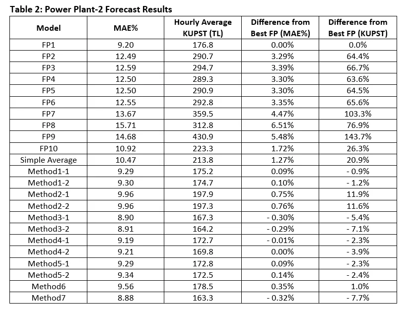
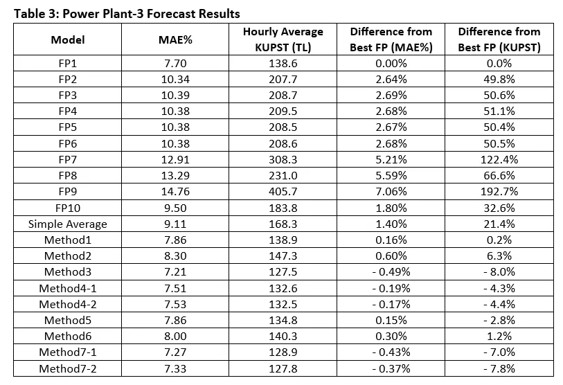
The MAE% and KUPST performances of the forecast providers (FP) and Ensemble Methods (along with the best model setups) are as follows in the tables below.
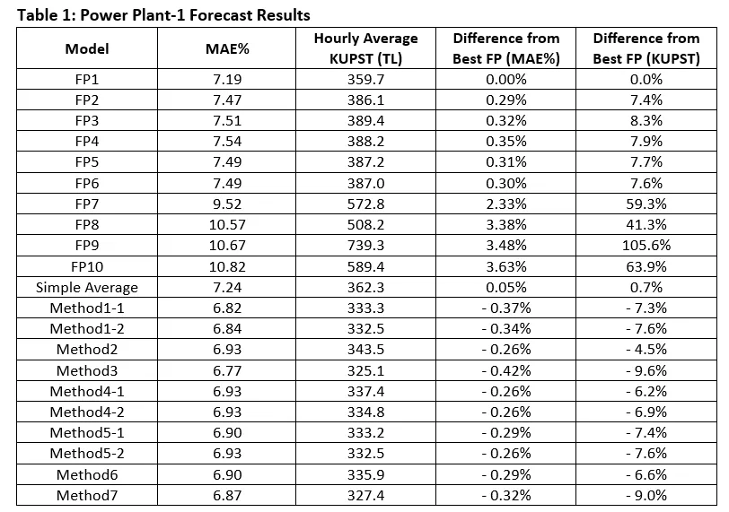
Note 1: MAE% results are calculated based on the most recent predictions made 70 minutes before the contract hour. For the KUPST calculation, predictions made both 70 and 40 minutes before were used.
Note 2: The best-performing method setup may differ for each power plant. For example, the setup of Method 2 in Power Plant 1 and 2 is different.
Note 3: For some methods, the setups that show the best performance in MAE% and KUPST criteria may differ, so results for two setups are shared for those methods.
By exploring the results in the tables, we can make the following conclusions:
- Ensemble Methods perform better considering the average performance in terms of MAE% and KUPST metrics.
- As highlighted in the previous article, we see once again that a model with higher accuracy does not necessarily yield better financial results. For example, when we look at FP7 and FP8 across all power plants, FP7 shows better performance in terms of MAE%, but FP8 shows better results in terms of KUPST.
- The simple average method which generally preferred as the main ensemble model in the market by the traders due to its simplicity, has significantly low performance compared to other Ensemble Methods across all power plants. The outcome can be used to emphasize the importance of choosing the possible best Ensemble Method among all others.
We can summarize the performances of Ensemble Methods and their potential returns compared to the best-performing base model, FP1, as shown at the table below. This table shows the results of the best-performing setup for each method for each power plant.
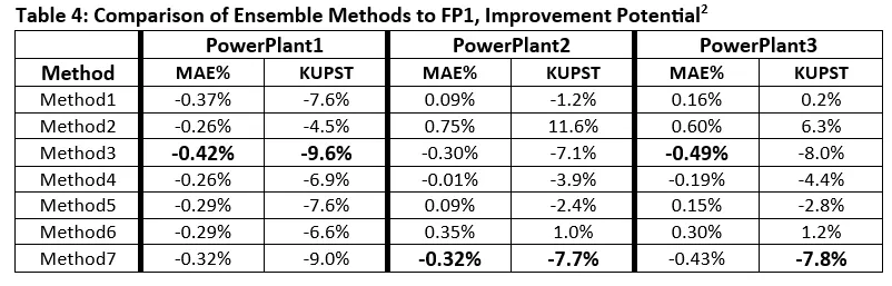
- When looking at the best-performing Ensemble Method for each power plant, these methods show results that are 0.42%, 0.32%, and 0.49% better in terms of MAE% compared to the best prediction provider, FP1.
- In terms of KUPST, the best Ensemble Methods have the potential to provide costs that are 9.6%, 7.7%, and 7.8% lower, respectively.
- We observe that different Ensemble Methods perform better for each power plant. Additionally, for Power Plant 2 and Power Plant 3, some Ensemble Methods do not surpass FP1 even in their best setups. This highlights the importance of selecting the appropriate Ensemble Method for each specific power plant.
- Selecting the right Ensemble Method is crucial for achieving the highest performance, but choosing the correct model setup is also important. For instance, in terms of KUPST, for Power Plant 1, 11 out of 12 setups of Method 3 perform better than FP1, while 1 performs worse. In Power Plant 2, 17 out of 30 setups of Method 7 perform better than FP1, while 13 perform worse.
In summary, testing Ensemble Methods across different power plants has demonstrated the consistency of their success. Additionally, we see the importance of selecting both the appropriate Ensemble Method and the model setup for each specific power plant. By choosing the right Ensemble Methods and setups, we can potentially achieve an improvement of around 7–10% in KUPST costs.
[1] KUPST is the cost of deviation amount from the confirmed daily generation program. KUPST cost is calculated on power plant level.
- KUPST is calculated as follows:
- KGUP: Confirmed Daily Generation Program
- KUPSM: Deviation Amount from KGUP
- KUPSM =
- Max(0,Realized Generation — KGUP*(1+Tolerance)) if Realized Generation > KGUP
- Max(0,KGUP * (1-Tolerance) — Realized Generation) if KGUP > Realized Generation
- KUPST = KUPSM * Max(MCP,SMP) * 0.03
- MCP: Day Ahead Market Price (Market Clearing Price)
- SMP: Imbalance Market Price (System Marginal Price)
- Tolerance is 0.21 for Wind Power Plants
[2] Imbalance costs can still be used for portfolios with multiple power plants, but it requires another approach, which will also be discussed in the next article. For now, we’ll keep the coverage on power plant level.
Caner Kahraman, Ali Güleç, Cem İyigün