
Wind Power Plants in Turkey
Electricity generated from wind in Turkey plays a key role in reducing energy dependence by replacing electricity generated from imported products such as coal and natural gas. With rapidly increasing investments in recent years, the installed capacity of wind PPs reached 12 GW by the end of February 2024. In 2023, the share of electricity generated from wind PPs in total electricity generation was realized as 10.4%.
The Importance of Generation Forecast for Wind PPs
Due to the nature of wind, forecasting wind generation with zero error is nearly impossible. Therefore, deviations from the generation forecasts often establish an extra challenge for balancing the electricity grid.
Two cost items encourage market players to have more accurate forecasts: imbalance cost and the deviation amount from the confirmed daily generation program (KÜPST). In other words, to avoid penalty costs, Wind PPs need to have forecasts as accurate as possible.
Generation Forecasting and Forecast Providers for Wind PPs
There are several inputs required to create accurate generation forecasts for wind PP’s; for instance, among others, wind speed forecast for the height of the turbine can be a crucial input. In addition to wind speed, variables such as wind direction, temperature, pressure, precipitation, and some others can be determinants. Many of the forecast providers use these inputs next to several others to obtain better results. Yet though they have quite sophisticated models running on several inputs, it is quite difficult to assert that one provider outperforms the others in all time. Acknowledging this fact, most wind PPs owners try to increase forecast accuracy and reduce risks by obtaining several forecasts from different forecast providers compared to forecasts obtained from a single provider.
Creating Forecasts from Different Generation Forecasts (Ensemble Methods)
Let’s call the forecasts we obtain from different sources “base forecasts”. Using base forecasts, ensemble methods are used to generate a more accurate forecast. These methods can surpass the performance of the best base forecast and produce more accurate outcomes. The most important assumption and expectation here is that each base forecast carries different information and that in the process of combining these forecasts, they will complete each other’s weaknesses. If the performance of a base forecast is noticeably superior compared to others under all conditions (e.g., summer-winter, day-night, or low-high wind speeds), the probability of ensemble methods providing benefits will be low. It would be logical to use ensemble models in cases where there are multiple forecast sources, utilizing different models with distinct information.
Frequently preferred ensemble methods are Simple Average, Median, Winsorized Average, Trimmed Mean according to Performance, Weighting by Model Performance, Regression-Based Methods, and Machine Learning-Based Methods.
Wind PP Generation Forecast Ensemble Methods Study
We conducted a study to deliver more accurate forecasts by using ensemble methods.
The study includes a total of 7 different forecast providers. The study covers approximately 9000 hours between January 2023 and February 2024. Adjusted Mean Absolute Error (MAE%) was used to measure wind generation forecast performance. The reason for not using Mean Absolute Percentage Error (MAPE) is that it results in very high error rates in places where generation gets closer to zero.
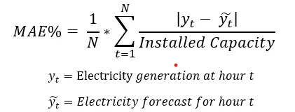
Forecast providers update their generation forecasts at different time frames. For a consistent comparison, the most recent forecasts provided at 40 and 70 minutes before the actual generation time were considered. The forecast given 70 minutes before the physical delivery provides a comparison point for Intraday trading, while the forecast given 40 minutes before provides a reasonable time point for KGUP revision which in the end is used to calculate KÜPST cost.
Except for simple averaging, other methods require a training period. Since the data is a time series, it makes sense to train ensemble methods with the most recent data. For this purpose, the training data was taken as the last 500 hours. The prediction period and training data followed a sliding window method with a window size of 100 hours.
The ensemble methods used in the study are:
- Simple average
- Trimmed mean according to performance (Selecting the best 2 base forecasts in the last 500 hours)
- Weighting by model performance (Weighting based on the cube of 1/MAE% in the last 500 hours)
- Weighting with linear regression
- Ensemble with the LGBM machine-learning model
The performances of forecast providers and ensemble methods in all test data after the first 500 hours are as follows in the table below. In the table, the performances of 7 forecast providers are ranked and shown as FP1, FP2…FP7.
FP1 represents smartPulse’s machine learning-based generation forecast model, Zada.
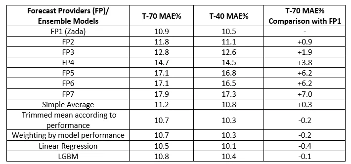
In the second and third columns, the MAE% values of the models’ predictions at T-70 and T-40 are respectively provided. In the last column, it shows how well the models perform based on the MAE% value of FP1, which is the best base forecast at T-70.
The top 2 models in the base models (with MAE% values of 10.9% and 11.8% at 70 minutes before and 10.5% and 11.1% at 40 minutes before) seem dominant. From FP3 onwards, it is noticeable that the performance of base forecasters is significantly lower compared to FP1, FP2, and ensemble methods. All ensemble methods outperform the base forecasts between FP2 and FP7. Only the Simple Average method shows poor results compared to FP1, while other ensemble methods perform better than FP1.
These results are quite motivating for implementing ensemble methods. However, an important question arises here.
Considering that the primary goal of a wind PPs owner company is to make a financial profit, is the model with the lowest MAE% really the most appropriate forecast for a wind PPs?
Here, the imbalance cost, the KÜPST penalty, and the market dynamics that determine these costs come into play. Let’s look at them now.
Cost-Based Performance Metric – Cost of Prediction Error (CPE)
The cost we evaluate as the imbalance cost is not calculated per power plant but for a portfolio of a Market Participant (MP) instead. When calculating the cost of imbalance for an MP, the aggregated forecast error of all plants and consumption portfolios should be taken into account to some extent. However, in this study, since we wanted to convey the idea in the simplest form possible, we assumed that each wind PPs would create a portfolio on its own. On the other hand, the KÜPST is a power plant-based penalty item, so there was no need to make any kind of simplification for this item.
The imbalance cost for a wind PPs is very roughly the penalty amount paid for the difference between the realized generation and the planned generation. The cost of imbalance depends on the total deviation amount (forecast error), the direction of error, the Market Clearing Price (PTF) of electricity in the Day-Ahead Market, and the System Marginal Price (SMF) in the Balancing Power Market and is calculated separately for each hour. The calculation is as follows:
- Energy Imbalance Volume (EDM) = Realized Generation + (Day Ahead Market Buy Volume + Intraday Market Buy Volume + Bilateral Agreement Buy Volume) — (Day Ahead Market Sell Volume + Intraday Market Sell Volume + Bilateral Agreement Sell Volume)
- If the imbalance volume (EDM) < 0:
- The MP pays an amount equal to max(PTF,SMF)*1.03*the imbalance volume
- If the imbalance volume (EDM) > 0:
- The MP receives payment equal to min(PTF,SMF)*0.97*the imbalance volume
When a generation higher than the planned happens, (when EDM is greater than zero) even though a payment is received, a cost is suffered. This cost is associated with selling electricity at a lower price than the price that was not sold in the Day-Ahead Market. The cost can also be considered as an opportunity cost.
The direction of forecast error, the difference between PTF and SMF can be crucial in the determination of the magnitude of the imbalance cost. The difference between the forecasts and the realized generation, due to several reasons which will be touched on in detail at the section where the model results are explained, does not create a symmetrical cost distribution function.
We estimated a hypothetical lumpsum and hourly average costs based on the forecasts we have obtained from each provider for the times t-70 and t-40. Using the forecast we had at t-70, we calculated the intraday trading volumes, and using the t-40 forecasts we achieved revised KGUP values. We assumed that all trades would be done over the weighted average prices that happened on each contract at the last 60 minutes. On top of these assumptions, we calculated the imbalance volumes for each contract so the imbalance costs and KÜPST penalty costs.
The total cost arising from forecast errors is the sum of the Imbalance and the KÜPST cost. Let’s call this the CPE (Cost of Prediction Error). So now, we have a cost-based performance metric. We’ll use this metric to increase the number of ensemble models from 5 to 7. The models that will use this metric will be Trimmed Mean wrt Performance and Weighting by Model Performance Ensemble Methods.
The hourly average CPE values for forecast providers and ensemble methods in TL are as follows:
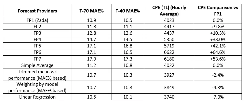
The fourth column indicates the hourly average of Imbalance cost and KÜPST combined. In the fifth column, there is a performance evaluation made of the CPE by comparing the results obtained for FP1 with all other providers and methods.
The results indicate that ensemble methods can create better results based on MAE%. Though FP1 model seems to be differentiated from the others when things comes to evaluating the results over MAE%, it seems like ensemble methods have the potential to outperform FP1. What is more remarkable is that all ensemble methods outperformed all providers over CPE values. Even the “Simple Average” method, which has the highest CPE value among ensemble methods, has the same CPE value as the best base model, FP1. The “Weighting by Model Performance (based on CPE)” method, which does not surpass FP1 in terms of MAE%, gives the lowest CPE result among all methods.
When comparing the performances of ensemble methods, as mentioned above, the “Weighting by Model Performance (based on CPE)” model gives the best result in terms of CPE, while “Linear Regression” provides the best result in terms of MAE%. “Linear Regression” outperforms all base models, and the CPE value of this method is close to the best ensemble method; “Weighting by Model Performance (based on CPE)” but only 16 TL/hour worse. While all ensemble methods except the “Simple Average” model improve the prediction performance by more than 2.5% compared to the best individual prediction model FP1 in terms of CPE, “Linear Regression” and “Weighting by Model Performance (based on CPE)” methods stand out with improvements of 7% and 7.4%, respectively.
It’s important that minimizing the MAE% does not necessarily mean minimizing the CPE. A forecast with a poor MAE% can yield better results in terms of CPE. For example, although the MAE% of FP7 is 0.8% worse than FP6, its CPE is 440 TL/hour worse. We see a similar situation in ensemble methods. Although the MAE% value of the “Linear Regression” method is the smallest, it does not provide the smallest CPE. While the “Trimmed Mean according to Performance” and “Weighting by Model Performance (based on MAE%)” ensemble methods have the same performance in terms of MAE%, the “Weighting by Model Performance (based on MAE%)” method provides better results in terms of CPE.
Although the ensemble method using LGBM machine learning produces better results both in MAE% and CPE compared to all forecast providers, it does not surpass the performance of linear regression. Model performances can be improved by trying different machine-learning models and hyperparameters. However, since the problem can be modeled quite efficiently with linear regression models, there may not be a need to dig in deep to explore possible value adds for different machine learning models and hyperparameters. Yet this can still be considered as something to explore in future works.
Finally, we think it’s worth mentioning that, compared to the second best provider FP2 (the best provider was smartPulse’s machine learning model so we believed it would be more convenient to compare with FP2 instead), there is potential for 6 million TL per year (ca 200.000 US$) saving when the ensemble method with the best CPE is utilized.
When we investigate the relationship between MAE% and CPE, we see that the asymmetric distribution of the PTF/SMF ratio plays a significant role. Energy deficits in most of the cases seemed to dominate the whole system for the period we studied, and it looks like it will be the case for the forthcoming months. Thus, at those times, when PTF starts to get closer to its upper limit and shows the tendency to stay there for a while, (where the system has a deficit) it might be better to have a positive Imbalance volume, acknowledging that the PTF/SMF distribution rather be skewed due to upper price limit of PTF and its distance to this limit.
In other words, in cases where the PTF/SMF ratio is low (SMF is higher than PTF), models that create comparably lower forecasts, create also lower CPE values. The fact that SMF is higher than PTF in many cases financially rewards lower generation forecasts. Because when we forecast low generation, the deviation amount is positive, we are selling at a value close to PTF with min(PTF, SMF)*0.97 in most cases. However, when the deviation amount is negative, we are paying at a value close to SMF with max (PTF, SMF)*1.03 in most cases.
In summary:
- Ensemble methods in wind PP generation forecasting have yielded decent results in improving base models obtained from forecast providers.
- Using the model that predicts generation the best does not necessarily mean it will produce the best financial results.
- The ensemble method, weighted by the CPE value of the models, has produced the best financial outcome.
- It should be considered that deliberately forecasting generation below or above, depending on the PTF/SMF ratio, may vary periodically and imply certain risks.
To elevate this study to the next level, the following steps can be considered:
- The number of power plants used in the study can be increased to test the consistency of the models.
- The number of machine learning models can be increased, and hyperparameter selection optimization can be done more systematically.
- Ensemble methods that produce portfolio-based forecasts for the imbalance cost can be developed instead of plant-based ones.
Caner Kahraman, Ali Güleç, Cem İyigün