
In our previous article, we discussed our efforts to enhance the accuracy of plant-level generation forecasts and reduce KÜPST costs using Ensemble Methods. In this article, we will delve into the portfolio management approaches we developed using the same techniques.
We understand the critical importance of accurately forecasting plant-level generation. However, beyond plant-specific decisions, it is often necessary to make different decisions at the portfolio level, as plant-level solutions may not always yield the best results for the portfolio as a whole. Table 1 clearly illustrates this concept with numerical data.
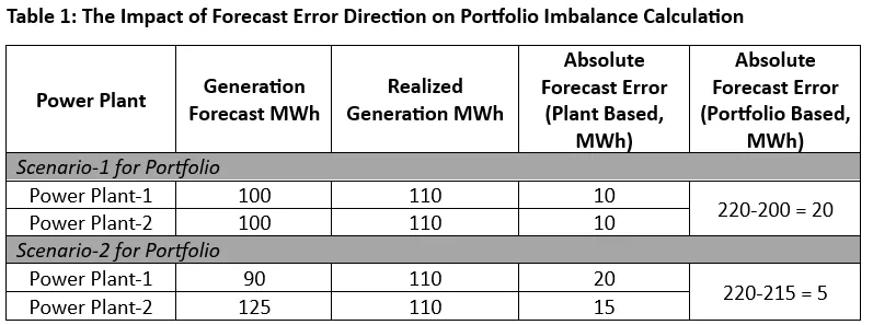
In the first scenario, the best forecasts are used for both plants, while in the second scenario, forecasts that are less accurate on a plant-specific basis compared to the first scenario are employed. In Scenario 1, the forecasts are 10 MWh below the actual generation, whereas in Scenario 2, the forecast for Plant-1 is 20 MWh below, and for Plant-2, it is 15 MWh above the actual generation.
Despite the deterioration in plant-specific forecasts, the total deviation for the portfolio in Scenario 1 is 20 MWh, while in Scenario 2, this deviation is only 5 MWh. This is because, in Scenario 2, the upward and downward deviations cancel each other out, resulting in a more accurate total generation forecast for the portfolio compared to Scenario 1.
This demonstrates that the direction of forecast errors for individual plants plays a critical role in determining the overall portfolio imbalance.
Therefore, the best forecast that minimizes KÜPST costs at the power plant level may not necessarily be the best forecast for the portfolio.
In this study, various combinations of forecasts generated using Ensemble Methods were utilized to reduce portfolio imbalance costs. The primary goal of creating these combinations was to leverage asymmetry in forecast deviations to identify the combination that minimizes total deviation. The sum of the three selected forecasts in each combination was treated as the total electricity generation forecast for the portfolio. Based on these forecasts, it was assumed that Day-Ahead Market (DAM) and Intraday Market (IDM) transactions would be carried out, and imbalance costs were calculated based on actual generation.
As a financial metric, the study employed the Cost of Prediction Error (CPE) metric, which includes the transaction values from the DAM and IDM, as well as the Energy Imbalance Cost, as previously detailed in earlier articles.
The study considered a total of 233 different forecasts for a single plant, comprising 223 different Ensemble Methods and 10 baseline forecasts. These forecasts were ranked and numbered based on their KÜPST costs. To ensure clarity and ease of understanding, the portfolio combinations were labeled as (t1, t2, t3), where:
- t1 represents the most accurate t1-th forecast for Plant 1,
- t2 represents the most accurate t2-th forecast for Plant 2, and
- t3 represents the most accurate t3-th forecast for Plant 3.
For example, a combination using the most accurate forecast for Plant 1, the 4th most accurate forecast for Plant 2, and the 7th most accurate forecast for Plant 3 would be labeled as (1,4,7).
Baseline forecasts, representing the currently used forecast providers, were labeled using the format FPX. For instance, if the baseline forecast 1 for Plant 1, baseline forecast 2 for Plant 2, and baseline forecast 4 for Plant 3 were used, the combination would be labeled as (FP1, FP2, FP4).
Initially, a 10x10x10 combination was created exclusively for the baseline forecast providers. Table 2 presents the CPE results for some of these combinations.
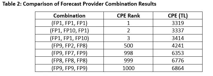
The combination consisting solely of forecasts from the provider that delivers the best results for each individual plant (FP1, FP1, FP1) has also produced the lowest Cost of Prediction Error (CPE) value for the portfolio. Table 2 presents the CPE values and rankings of several baseline forecast combinations among all possible combinations.
At this point, it seems that using the forecasts that yield the best results for individual plants also provides the best results for the portfolio. But what if we conducted a similar analysis using Ensemble Methods?
When evaluating all possible combinations involving Ensemble Methods – a total of 11.1 million combinations (223x233x223) – the results are as shown in Table 3.
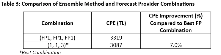
Examining the results in Table 3, we see that the optimal portfolio combination involves using the forecast that produces the best KÜPST result for Plant 1 and Plant 2, and the third-best KÜPST result for Plant 3. This combination outperforms the best baseline forecast provider combination by 7%.
Generating all possible combinations and calculating their CPE values took approximately one day using Python. As the number of plants and Ensemble Methods increases, the computation time grows exponentially. For example, adding one more plant to the current hypothetical portfolio would increase the total number of combinations by 233 times. Given the number of plants typically found in portfolios in our market, it becomes clear that testing all possible combinations is practically impossible. Therefore, finding the optimal combination – or those with near-optimal performance – within a reasonable computation time is of critical importance.
To address this challenge, subsets containing fewer Ensemble Methods were analyzed. These subsets were derived by selecting the top K Ensemble Methods for each plant based on their KÜPST results, creating a smaller pool of combinations to evaluate.
When K was set to 1, using the best KÜPST-producing Ensemble Method for each plant, the (1,1,1) combination delivered results that were 6.5% better than the best baseline forecast combination according to the CPE metric. Moreover, the (1,1,3) combination – where the best Ensemble Method for Plant 3 was not used – showed an improvement of 7%. This further highlights the potential of exploring different combinations to achieve better results.
To evaluate how results vary with different subset sizes, combinations were created with K values of 20, 50, and 100 (20x20x20, 50x50x50, and 100x100x100). A comparison of results and computation times for these subsets is presented in Table 4.
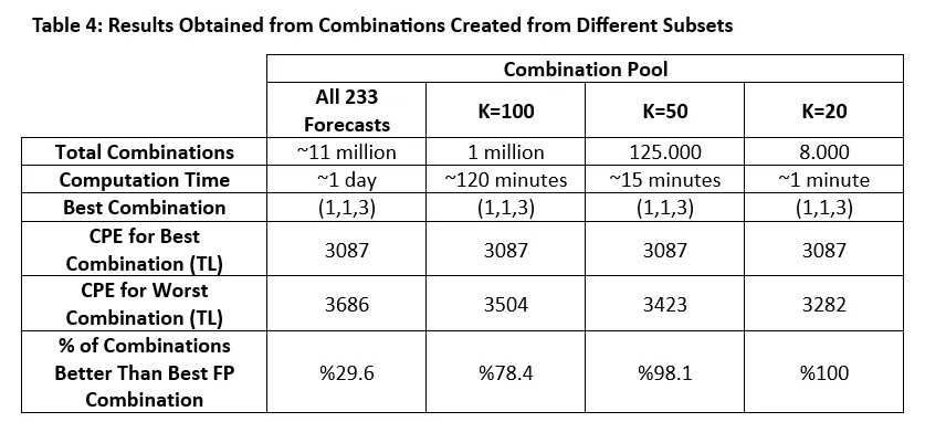
The best combination remained consistent across different subsets of combinations. When considering computation times, it becomes evident that testing all possible combinations is unnecessary. For instance, while evaluating the 50x50x50 subset took approximately 15 minutes, the 20x20x20 subset was completed in less than a minute.
Beyond identifying the best Ensemble combination, we also examined the percentage of combinations within each subset that outperformed the best baseline forecast combination. The results show that as the subset size decreases, the percentage of better-performing combinations increases. For example, 98% of the 50x50x50 combinations performed better than the best baseline forecast combination. As expected, reducing the value of K results in a pool of combinations with more similar CPE values.
When analyzing the 20x20x20 combination pool, we observed that every solution in this subset outperformed the best baseline forecast combination. Furthermore, any solution within this subset achieved results close to the best Ensemble combination, (1,1,3), in terms of CPE (TL). In summary, calculating all possible combinations to find the best Ensemble combination is unnecessary. Instead, working with a small subset of Ensemble Methods that produce the best KÜPST results for each plant appears to be sufficient. In fact, the combination of the top KÜPST-producing Ensemble Methods, (1,1,1), deviates from the best combination by only 0.5%.
Another alternative could involve grouping Ensemble Methods into categories and selecting the best methods from each category for each plant. This approach would increase the diversity of methods within the combinations. As a reminder, the categories include:
- MAE-based
- KÜPST-based
- Regression-based
- Machine Learning-based
- Regression + SMP/MCP adjustment
When the top 3 methods from each category – 15 methods in total – are analyzed, resulting in 15x15x15 (a total of 3,375 combinations), the outcomes are as shown in Table 5.
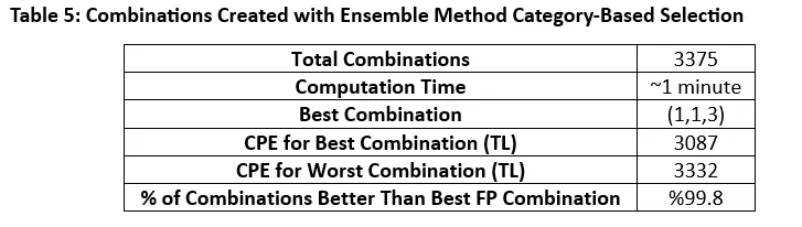
When category-based selection is applied, the best combination is achieved in under one minute of computation time, with 99.8% of all combinations outperforming the baseline forecast combinations. An interesting finding is that the worst CPE value in the scenario where the top 20 Ensemble methods for each plant were crossed (as shown in Table 4) is better than the worst CPE value among combinations formed by selecting methods from different categories. Additionally, the variability in CPE values among combinations formed from the best-performing methods for each plant is noticeably lower.
Key Findings:
- The use of plant-specific Ensemble Methods has proven effective in significantly reducing KÜPST costs. Furthermore, portfolio management based on these combined forecasts has demonstrated notable success in reducing imbalance costs.
- Using the best forecasting methods for individual plants may not necessarily yield the best results at the portfolio level. Forecasts optimized for individual plants do not always lead to optimal portfolio performance, underscoring the importance of portfolio-based combination strategies.
- In scenarios with a high number of combinations, selecting subsets to reduce computation time is crucial. This method minimizes the risk of overlooking the best or sufficiently good forecasts, ensuring gains in computational efficiency without sacrificing forecast accuracy.
- While combining plant-specific forecasting models can help reduce imbalance costs by selecting the best fit for the portfolio, alternative approaches could focus on directly producing forecasts optimized for the entire portfolio. Some of these approaches will be explored in our next article.
These findings highlight the value of combining plant-level forecasts while considering broader portfolio-level strategies to achieve optimal results.
Caner Kahraman, Ali Güleç, Dr. Cem İyigün